CAT Quant: Statistics – Important Formulas and Concepts
Introduction
- Statistics deals with collection, classification, presentation, analysis and interpretation of numeric data (quantitative data).
- The quantitative data occurs in three forms namely
- Individual series
- Discrete series
- Continuous series.
Measures of Central Tendencies
- A measure of central tendency indicates the central value of the size of a typical member of the group
- Various measures discussed under central tendency are –
- Arithmetic Mean
- Geometric Mean,
- Harmonic Mean
- Median
- Mode
Arithmetic Mean (A.M.) \( (\bar{x}) \)
- Given x1, x2, x3, ….. xn (n individual items), then – $$AM= \overline{x} = {\LARGE [} \ \frac{x_{1}+x_{2}+x_{3}…+x_{n}}{n} \ {\LARGE ]} \\ \overline{x} = \frac{Sum \ of \ the \ observations}{The \ number \ of \ observations}$$
- For Example : The arithmetic mean of (4, 7, 8, 14, -13) is – \( \frac{4+7+8+14+(-13)}{5}=\frac{20}{5}=4 \)
- The algebraic sum of deviations about the mean is 0 or \( \Sigma(x-\overline{X})=0 \)
- The arithmetic mean to two numbers a, b is \( \frac{a+b}{2} \)
- For an AP series, AM is the arithmetic mean of equidistant terms.
- If b = AM of (a,c) then a, b and c are in arithmetic progression.
Geometric Mean (G.M.)
- Given x1, x2, x3, ….. xn (n individual items all being positive), then $$GM=\sqrt[n]{(x_{1}*x_{2} *…….*x_{n})} \\ GM = n_{th} \ root \ of \ the \ product \ of \ the \ numbers$$
- For Example – The geometric mean of (50, 100, 200) is \( \sqrt[3]{(50\times100\times200)} = \sqrt[3]{(1000000)} = 100 \)
- The geometric mean of two positive numbers a, b is \( \sqrt{ab} \)
- If b=GM of (a,c), then a, b and c are in geometric progression.
Harmonic Mean (H.M.) –
- Given x1, x2, x3, ….. xn (n individual observations such that none of them is equal to 0), then $$HM=\frac{n}{\frac{1}{x_{1}}+\frac{1}{x_{2}} + \frac{1}{x_{3}} +………….+\frac{1}{x_{n}}} $$
- For Example : The harmonic mean of (2, 4, 6, 8, 10) is \( \frac{5}{\frac{1}{2}+\frac{1}{4}+\frac{1}{6}+\frac{1}{8}+\frac{1}{10}} = \frac{5 \times 120}{60+30+20+15+12} =\frac{600}{137} \)
- HM of two numbers a, b is \frac{2ab}{a+b}
- If b=HM of (a,c), then a, b and c are in harmoni progression.
NOTE : For any two positive numbers a, b $$ AM \ge GM \ge HM \\ (GM) = \sqrt{ (AM) \times (HM)}$$
Median
- The median is the middle value of a dataset when it is arranged in ascending or descending order.
- If the dataset has an odd number of values, the median is the middle value. For Example : The median of (five values) \( 4, 7, 12, 15, 20 \ \ is \ \ 12\) .
- If the dataset has an even number of values, the median is the average of the two middle values. For Example : The median of \( 3, 5, 9, 11, 13,15 \ \ is \ \frac{9+11}{2}=10\)
- The median divides the distribution into two equal parts.
- Median is suitable for qualitative data as well.
Mode
- The is the item which is most often found in the given set of observations, Le, the value occurring the highest number of times.
- A dataset can have one mode (unimodal), more than one mode (multimodal), or no mode if all values are unique.
- For the observations – 2, 1, 1, 2, 3, 4, 3, 2, 1, 2, 2, 1, 4,6,7 : Mode = 2
- For the observations – 5, 7, 11, 25, 36, 16. Here no item occurs more than once. So, mode is Ill-defined.
Empirical Formula
- \( Mode = 3Median \ – \ 2Mean \)
- This formula is valid for the distribution which are moderately symmetric. (symmetry being coincidence of mean, median arid mode)
Measures of Dispersion
- A measure of dispersion indicates the extent to which the different items of the group are spread about the average.
- Various measures discussed under dispersion are –
- Range
- Quartile Deviation
- Mean Deviation
- Standard Deviation/Variance.
Range
- Given x1, x2, x3, ….. xn (n individual observations) $$ Range = [ \ maximum \ value \ – \ minimum \ value \ ]$$
- For Example : Range of \( [7,4,8,1,6,11,15] = (15-1) = \ 14 \)
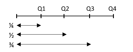
Quartile Deviation (Q.D.) or Semi Inter Quartile Range
- Quartiles are those values, which divide the distribution into four equal parts, when the values are arranged in ascending or descending order of magnitude. \( \\ \)

- Q1 called the first quartile, Q2 is the middle quartile and Q3 the third quartile. The second quartile is also referred to as the median.
- As the name semi-inter-quartile range itself suggests $$ QD =\frac{Q_{3}-Q_{1}}{2} \ [one-half \ the \ range \ of \ quartiles]$$
- For calculation –
- Q1 = size of \( {\LARGE(} \frac{n+1}{4}{\LARGE)}^{th} \ term \)
- Q3= size of \( 3{\LARGE(} \frac{n+1}{4}{\LARGE)}^{th} \ term \)
- Note : The data is not in the ascending order (or in the descending order). So we arrange it first and then proceed.
- For Example : Find the QD of the observations 5, 9, 13, 15, 21, 23 and 25 \( \\ Q_1 = {\LARGE(} \frac{7+1}{4}{\LARGE)}^{th} \ term = 2^{nd} \ term = 9 \\ Q_3 = 3{\LARGE(} \frac{7+1}{4}{\LARGE)}^{th} \ term = 6^{th} \ term = 23 \\ thus, \ QD = \frac{Q_{3}-Q_{1}}{2} = \frac{23-9}{2} = 7\)
Mean Deviation (M.D.)
- The mean deviation is calculated about mean or median or mode. But by default mean deviation is about mean.
- Mean deviation is the average of deviations of each item in the data set from the mean. $$MD=\frac{\sum_{i=1}^{m}|x_{i}-A|}{n} \\ A = mean / median / mode \ ; \ n = number \ of \ items$$
- For Examples : Find the mean deviation of 2, 5, 9, 11, 13 – \( \\ Mean \ of \ the \ observations \ \overline{x} = \frac{40}{5} = 8 \\ thus \ , \ MD = \frac{|2-8|+|5-8|+|9-8|+|11-8|+|13-8|}{5} =\frac{6+3+1+3+5}{5}=\frac{18}{5}=3.6 \)
- Mean Deviation of two numbers a, b = \( \frac{|a-b|}{2}\)
- Mean deviation is based on each and every observation.
Standard Deviation (S.D.)
- Standard quantifies the amount of variation or dispersion from the average (mean) of the dataset.
- A low standard deviation indicates that the data points tend to be close to the mean, while a high standard deviation indicates that the data points are spread out over a wider range of values.
- Standard Deviation is the root mean squared deviation taken about the mean. $$SD= \sqrt{\frac{\Sigma(x_{i} – \overline{x})^{2}}{n}}, \ where x_1, x_2, x_3, ….. x_n \ are \ the \ items \ given. \\ The \ expression \ \sqrt{\frac{\Sigma(x_{i} – \overline{x})^{2}}{n}} \ also \ equals \ to \ \sqrt{\frac{\Sigma{x_{i}}^{2}}{n}-(\overline{x})^{2}} $$
- For Example : Find the standard deviation of (2, 5, 7, 10, 13, 17) – \( Mean \ of \ the \ observations\ \overline{x} \ = \frac{54}{69} = 8 \\ thus, \ SD = \sqrt{\frac{\sum(x_{i}-\overline{x})^{2}}{n}} =\sqrt{\frac{(-7)^{2}+(-4)^{2}+(-2)^{2}+(1)^{2}+(4)^{2}+(8)^{2}}{6}} =\sqrt{\frac{49+16+4+1+16+64}{6}}=\sqrt{\frac{150}{6}} =\sqrt{25}=5 \)
- The square of the standard deviation is variance.
- The standard deviation is always non-negative.
Read concepts and formulas for: Time and Work
Read more about AI practice Platform here: https://www.learntheta.com/cat-quant/